Trigonometry

This is a brief tutorial with examples of how to use some of the trigonometry and math functions in p5js.

These are the basic trigonometric functions (and the Pythagorean theorem) that relate the angles of a right triangle to the lengths of its sides:

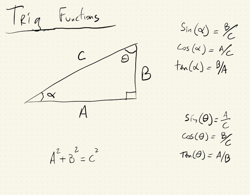
These can be used to derive formulas for translating between Cartesian and polar coordinate systems.

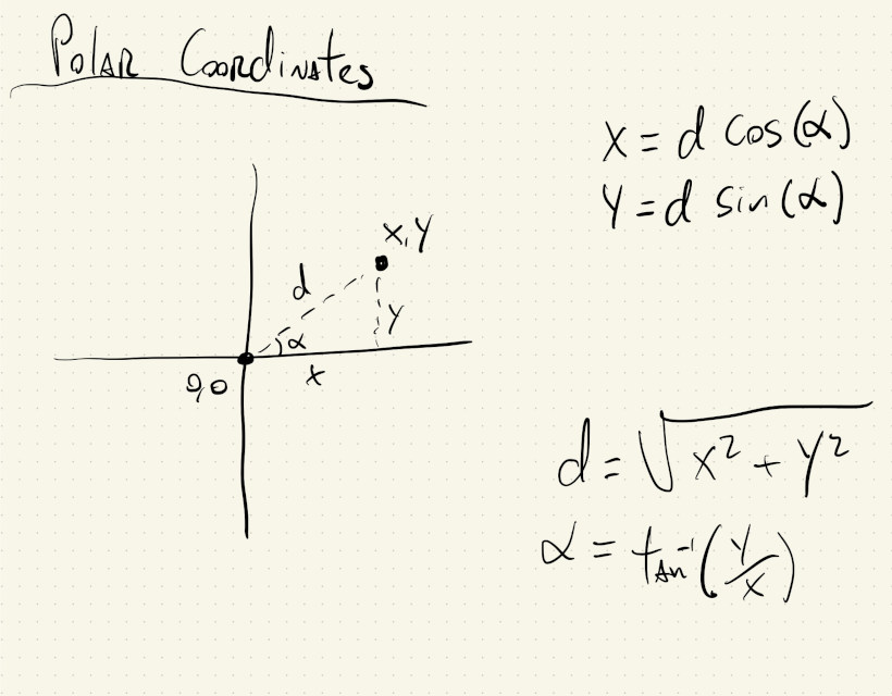
Cartesian coordinates are what we use to specify points on a plane (and pixels on a screen) using two numbers that represent distances in perpendicular directions. Polar coordinates specify points on a plane using a distance and an angle.

Just like we can use for() loops to iterate over \(2\) cartesian coordinates \((x, y)\) and create patterns in a grid, we can also iterate over the \(2\) variables in a polar coordinate system to create patterns:

This one is pretty simple and could’ve been done by drawing concentric ellipses.

And that’s basically what the for() loops are doing: as long as we keep the angle used to calculate \(x\) equal to the angle used to calculate \(y\), we get circles.

But, what if we move the \(x\) angle \(3\) times faster than the \(y\) angle?

If we just change this:

let x = r * cos(radians(a));

to this:

let x = r * cos(radians(3 * a));

we get this:

Yeah… polar coordinates FTW! I don’t think we can draw that with circles.

We can play with that value and see how the drawing changes. We can also add a different multiplier to the \(y\) angle as well:

let x = r * cos(radians(3 * a));
let y = r * sin(radians(7 * a));

Or, use something else, like the \(r\) value, to increment the angle:

let x = r * cos(radians(a + 2 * r));
let y = r * sin(radians(a));

Or, both:

let x = r * cos(radians(2 * a + 2 * r));
let y = r * sin(radians(a));

We can also derive the \(r\) and \(a\) angles from the same for() loop variable.

If we make \(r\) grow proportional to the angle, we get a spiral:

And if we increase the frequency of the angles like we did before, and also increase the range of our \(r\):

let r = map(a, 0, 360, 10, 0.7 * width);
let x = r * cos(radians(6 * a));
let y = r * sin(radians(6 * a));

We get a tighter spiral that goes all the way to the corners of our canvas:

We can add an offset to our angles (this is often called the phase of an angle):

let x = r * cos(radians(6 * a - frameCount));
let y = r * sin(radians(6 * a - frameCount));

And, if that offset increases or decreases with every frame, we get a hypnotizing animation:

Our canvas is spinning slowly, but the shape makes it seem like it’s a line that is being drawn infinitely, or circles that are growing.

We can make it go faster by multiplying frameCount by a constant, like:

let x = r * cos(radians(6 * a - 8 * frameCount));
let y = r * sin(radians(6 * a - 8 * frameCount));

And if we make the the \(x\) and \(y\) angles slightly out of sync:

let x = r * cos(radians(7 * a - 8 * frameCount));
let y = r * sin(radians(6 * a - 8 * frameCount));

we get an effect that is almost 3D:

And, finally, we now understand equations like this and can code them into our sketches: \(\begin{align*} x &= 16 * sin^3(t) \\ y &= 13 * cos(t) - 5 * cos(2t) - 2 * cos(3t) - cos(4t) \end{align*}\)

\(t\) is the angle, which, in our case, goes from \(0^\circ\) to \(360^\circ\):

Pretty cool!

Polar coordinates are lots of fun, and can also be very useful when we need to calculate the distance or the angle between two points.

If we image two points on our screen, with coordinates \((x_0, y_0)\) and \((x_1, y_1)\), we can get the distance between them by using the Pythagorean theorem:

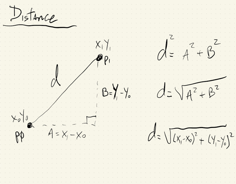
In this sketch the distance between two moving points is calculated using the formula \(\sqrt{(x_1 - x_0)^2 + (y_1 - y_0)^2}\) and the p5js function dist(). When those distances are used as the diameter for two circles centered on the canvas, we can see that they are exactly the same:

Similarly, we can use the formula that calculates the polar angle of a point to get the angle between two points:

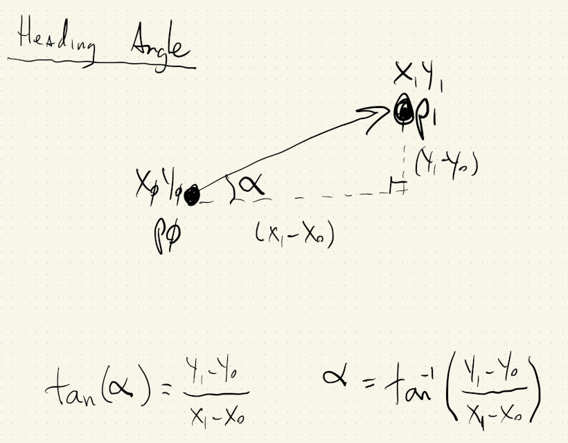
Or, the angle between a point and itself in the future.

If a moving point at \((x, y)\) has velocity \(v_x\) and \(v_y\), its position in the near future will be \((x + v_x, y + v_y)\). We can calculate the angle between the point now and the point in the future to get its heading angle:

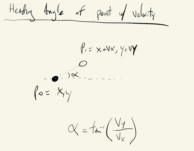
We can use the heading angle of a moving object to rotate its shape and emphasize its direction of motion:

While not as common, sometimes we might want to calculate the distance between a point and a line.

This is the shortest distance from a given point to any point on an infinite straight line. It is the perpendicular distance of the point to the line, or, the length of the line segment which joins the point to nearest point on the line.

It’s distance \(d\) between \((X, Y)\) and the line \(y = \frac{m}{n}x + b\) on the drawing below:

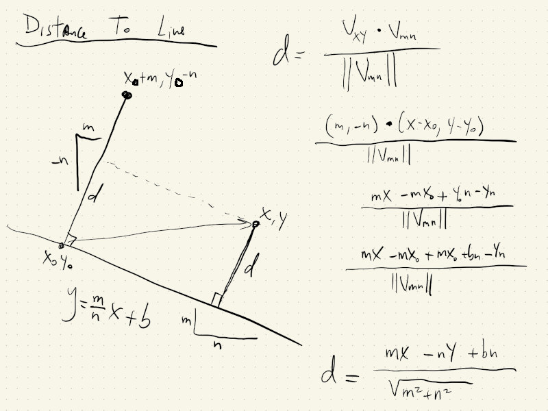
There are many ways to derive the equation for the distance. The one in the drawing involves using distances from another point \((X_0, Y_0)\), also on the line, to the original point and to a point \((X_0+m, Y_0-n)\) that is perpendicular to the line. The final distance equation is:

Again, the details of how this is derived are not super important. We should just know that it can be calculated, and that the equation is here in the tutorial whenever we need it.

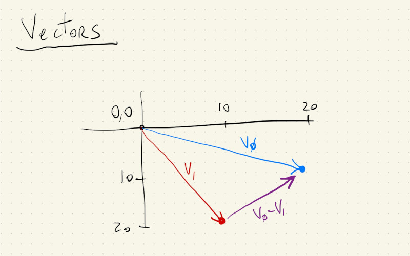
p5.js actually has a class called Vector that can help with geometry calculations like these. The simplest way to think about a vector is that it specifies a point \((x, y)\) in space, relative to the \((0, 0)\) origin. Vectors are actually more than that, but to do the distance and angle calculations that we’ve seen, it’s fine to think of vectors as points with an \((x, y)\) coordinate.

This drawing shows two vectors/points and if we subtract \(_1\) from \(v_0\), we get a third vector that holds information about the distance and direction between them.

The vectors in p5js actually have builtin functions to calculate distances and angles. We can create two vectors and get the distance between them like this:

let v0 = createVector(20, 10);
let v1 = createVector(10, 20);
let d = v0.distance(v1);

and the angle like this:

let v0 = createVector(20, 10);
let v1 = createVector(10, 20);
let d = v0.angleBetween(v1);

Let’s use vectors to redo some of the sketches in the tutorial.

First, distance:

Instead of pushing JavaScript objects with \(4\) parameters \((x, y, vx, vy)\), we now have objects with two vectors, one for the location and one for the velocity of the objects.

In draw, anytime we had p.x now we’ll have to use p.loc.x. Likewise for velocity, p.vx becomes p.vel.x. It might a bit more letters to type, but the related quantities are in a vector, which helps to do some math, like updating the location.

Instead of this:

p.x += p.vx;
p.y += p.vy;

We can just do:

p.loc.add(p.vel);

And the distance between the two circles can now be calculated with:

ps[0].loc.dist(ps[1].loc);

For the angles, it’s very similar. We can always call
v0.angleBetween(v1) to get the angle between two vectors. We just have to think about which \(2\) vectors we need the angle between.

In the example where we are trying to get heading angles, the vector that points in the direction of movement is p.vel. Since in p5js an angle of \(0^\circ\) points in the direction along the x-axis, the angle that we need to rotate our objects is gonna be relative to this reference vector of zero rotation.

The code is mostly the same as the previous sketch, with the vector addition for location updates, but now we do:

let xAxis = createVector(1, 0);
let hAngle = xAxis.angleBetween(p.vel);

This way we get the heading angles relative to the reference point of zero rotation, and then use that to rotate our objects.

To calculate the distance to a line, the code remains mostly the same, and it looks just as complicated, but in reality it uses some of the properties of vectors to make the calculation a little more geometric instead of algebraic, which can help remember how to derive the formula at a later time.

Again, don’t worry about the details for this one, just know where it it and how to use it.

We first define a line object with parameters for its equation in the form: \(y=mx + b\). We then use these parameters to create a vector that is perpendicular to this line, so we can project our original vector onto this perpendicular vector. And just like that, we get the distance.

Now that we know about classes, we can even create a class for the line with equation \(y = mx+b\) and keep all of the math for calculating distances inside the class:

This is one of the great things about classes: once we have the math for something figured out, we can always wrap it inside a class that will use it to update an object’s shape, color, position, etc, and then we can have \(10\) or \(100\) of these objects by just creating new instances from our class definition.

For example, we can move the color info inside our object, call it a Light class and use it to create a couple of lights in our canvas:

And now automate some slope changes over time, sit back and enjoy a low-fi, pixel light show: